Year 12 Physics Practical Investigation | Projectile Motion Experiment

Have a physics practical assessment task on Projectile Motion? Read this complete report on a common Year 12 Physics Projectile Motion Investigation.

Sample Physics Practical Assessment Task: Projectile Motion Experiment

Projectile motion experiment is used by most schools for their first Physics practical assessment task. This is because most Projectile Motion practical investigation is relatively easy to design and conduct by students.

A typical Projectile Motion practical assessment task used by schools is outlined below.

Task title

Task 1 of 4 Open-Ended Investigation Report on Projectile Motion from Module 5 Advanced Mechanics.

Task weighting

20% of Overall school assessment

Description of Assessment Task

Design and conduct a practical investigation to collect primary data to validate the relationship between the launch velocity and the range of a projectile.
Use the results to calculate the acceleration due to gravity.

In this sample practical assessment task, we are required to investigate the relationship between the range $s_x$ and the launch velocity of a projectile released from an elevated position.

Let’s apply the scientific method to design and conduct a practical investigation for the assessment task outlined above.

Sample Physics Practical Report

1. Theory

The simplest type of projectile motion is a ball being projected horizontally from an elevated position.

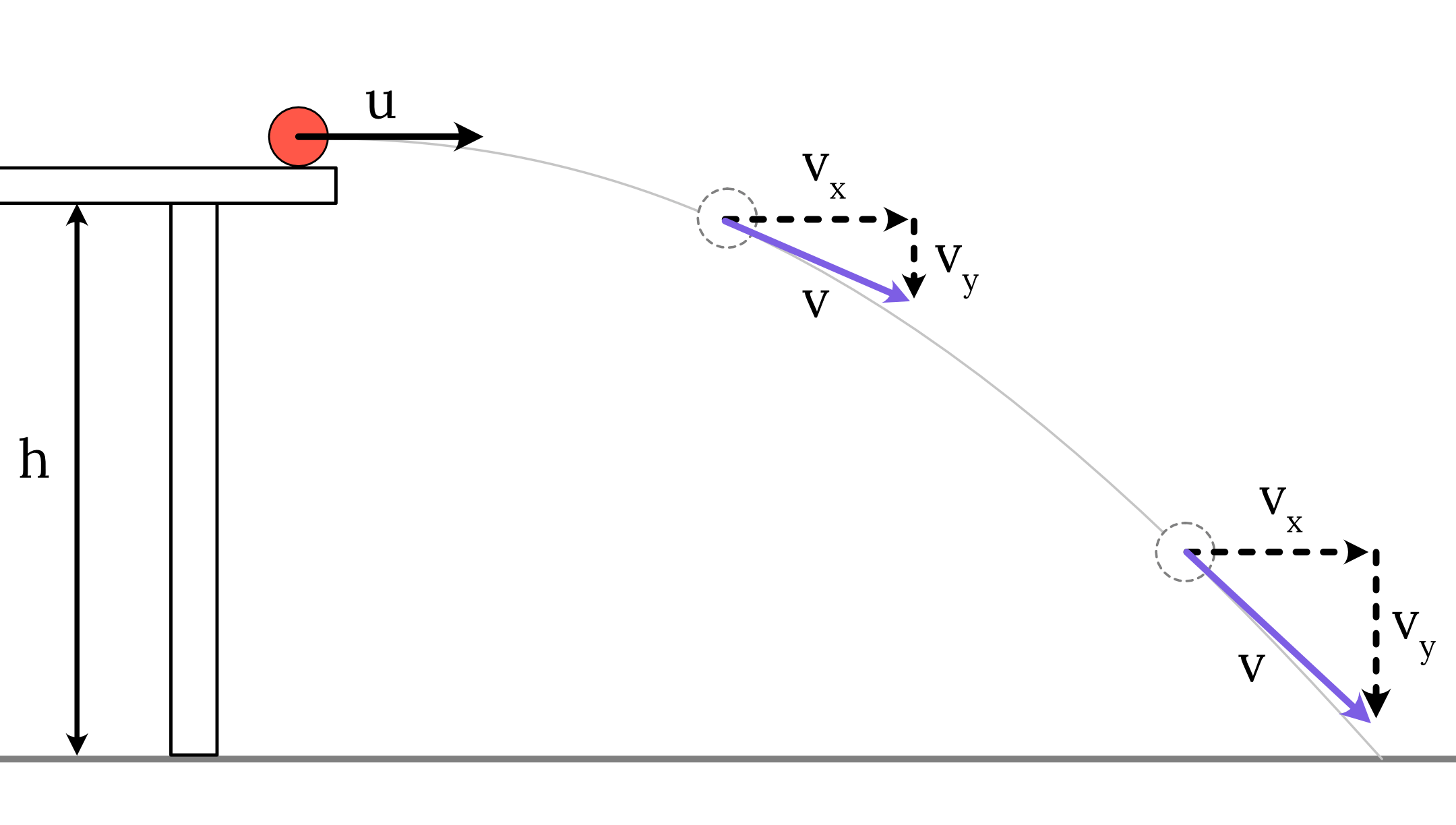
Guide - Physics Practical Investigation_Projectile motion

In this situation, the range of a projectile is dependent on the time of flight and the horizontal velocity. Hence this experiment is based on the equation $s_x=u_xt$ .

To express the time of flight $t$ in terms of the acceleration due to gravity, we analyse the vertical motion of the projectile

$s_y=u_yt+\frac{1}{2}at^2$

$-h=0+\frac{1}{2}(-g)t^2$

$t^2=\frac{2h}{g}$

$t=\sqrt{\frac{2h}{g}}$

Hence the range of a projectile can be expressed in terms of the horizontal velocity and the other control variables such as $y$ and $g$ by substituting $t=\sqrt{\frac{2h}{g}}$ expression into $s_x=u_xt$ :

$s_x=u_xt$

$s_x = u_x \times (\sqrt{\frac{2h}{g}})$

$\therefore s_x = (\sqrt{\frac{2h}{g}}) u_x$

2. Variables

Before designing your investigation, all the variables need to be identified.

Independent variable: Horizontal launch velocity $u_x$
Dependent variable: Range $\Delta x$
Control variables: Height of the table $y$ , acceleration due to gravity $g$ , the shape of the projectile

Keeping the control variables constant allows the experiment to be more valid.

To learn more about how to improve the validity of your experiment, read the Matrix blog on ‘Validity, Reliability and Accuracy of Experiments‘

3. Aim

To determine the relationship between the range of a projectile $\Delta x$ and its horizontal launch velocity $u_x$ and use the results to calculate the acceleration due to gravity $g$ .

4. Method

The apparatus is set up as shown in the diagram below.
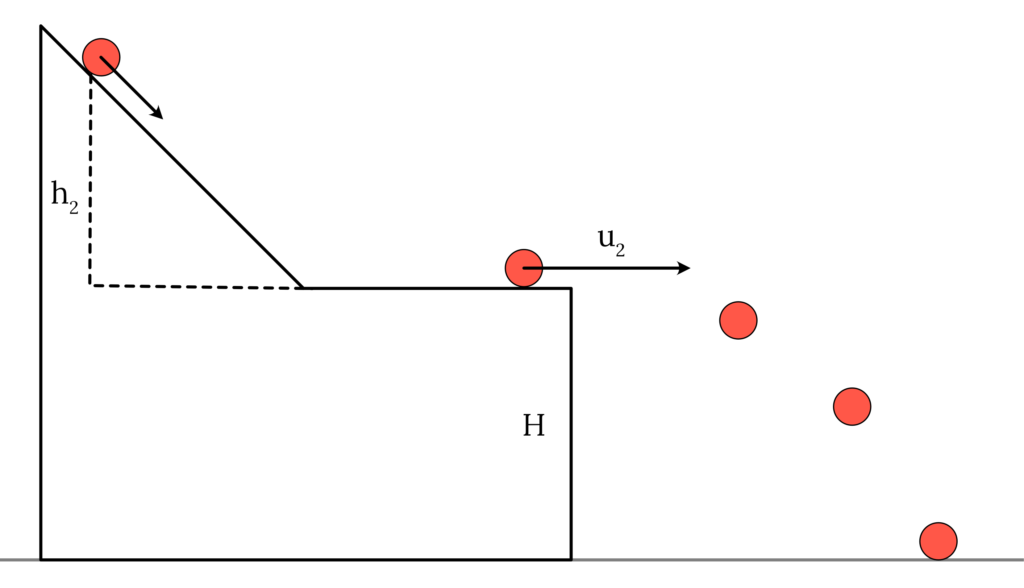
A smooth metal ball is placed at the top of the ramp, and the vertical distance from the ball to the table is measured.
The ball is rolled down and timed along the $1 \ m$ horizontal length using a stopwatch. The time is recorded.
The distance from the foot of the table to its landing point on the carbon paper is observed, measured and recorded.
Steps 1-4 are then repeated at different heights up the ramp.

5. Results

The results are given in the table below. Using the times taken for the ball to travel 1 metre. Data collected from the experiment is highlighted in blue.

Vertical height on ramp $\Delta h \ (m)$	Time to travel $1 \ m \ (s)$	Range $\Delta x \ (m)$
0.6	0.30	1.37
0.5	0.31	1.26
0.4	0.37	1.14
0.3	0.40	0.98
0.2	0.53	0.81

6. Quantitative Analysis of Results: Graphs and calculations

Calculate the horizontal velocity of the ball as it leaves the table and hence complete the table.

Vertical height on ramp $\Delta h \ (m)$	Time to travel $1 \ m \ (s)$	Launch velocity $u_x \ (ms^{-1})$	Range $\Delta x \ (m)$
0.6	0.30	$u_x = \frac {s_x}{ t}$ $u_x= \frac{1}{0.30} = 3.33$	1.37
0.5	0.31	$u_x= \frac{1}{0.31} = 3.23$	1.26
0.4	0.37	$u_x= \frac{1}{0.37} = 2.70$	1.14
0.3	0.40	$u_x= \frac{1}{0.40} = 2.50$	0.98
0.2	0.53	$u_x= \frac{1}{0.53} = 1.89$	0.81

Plot the range of the ball $\Delta x$ against the launch velocity $u_x$ and draw in the line of best fit.

The range of the ball is plotted against the horizontal launch velocity.

Graph

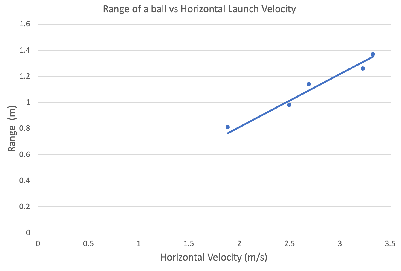
A line of best fit is drawn.

Determine the relationship between the launch velocity $u_x$ and the range of the ball $\Delta x$ and hence discuss its significance

The relationship between the launch velocity and the range of the ball is linear. The range of the ball is directly proportional to the horizontal launch velocity: $s_x = u_x \times t$
The linear relationship implies that the horizontal launch velocity affects the range but not the time taken to fall from a fixed height. Therefore horizontal and vertical motions are independent of each other.
This also validates the results expected from the equations of projectile motion.

Use the gradient to find the acceleration due to gravity

Action	Detail
Step 1: Find the gradient of the line of best fit.	Gradient can be determined from the graph. Gradient = $\frac{Rise}{Run} = 0.40$
Step 2: Identify the variables	Independent variable: Horizontal launch velocity $u_x$ Dependent variable: Range $\Delta x$ Control variables: Height of the table $y$ , acceleration due to gravity $g$ , the shape of the projectile
Step 3: Rewrite $\Delta x = (t) u_x$ in the form $y = (k)x$ to determine the relationship between the dependent, independent and control variables.	$\Delta x = u_x t$ $\Delta x = (t) u_x$ $\Delta x = (\sqrt{\frac{2H}{g}}) u_x$
Step 4: Write the gradient in terms of control variables.	Since $\Delta x$ is directly proportional to $u_x$ , the gradient equals to $\sqrt{\frac{2H}{g}}$
Step 5: Find the unknown in the control variable.	Using the launch height y = 0.7 m and the gradient, determine the acceleration due to gravity g. $gradient = \sqrt{\frac{2H}{g}}$ $g= {\frac{2H}{(gradient)^2}}$ $g= {\frac{2 \times 0.7}{(0.4)^2}}$ $g= 8.75 ms^{-2}$ The acceleration due to gravity is $-8.75 ms^{-2}$ downwards.

7. Qualitative Analysis: Evaluation of method and errors

Let’s investigate the errors, reliability and accuracy of this experiment.

Question	Answer
How would you determine if the results are reliable?	Reliability refers to how close the experimental results are to each other. In order to assess the reliability, we must consider the deviation of each point from the line of best fit. If the deviation is low, then the results can be considered reliable
Suggest a method of improving the reliability of your results.	Reliability here can be improved by taking repeated measurements at each of the vertical heights and using the average of these values when plotting the graph. Averaging will reduce the effect of random errors.
What are some potential errors in this experiment? How can these errors be reduced?	The main errors experienced in this experiment are: Errors associated in measurement of time to travel 1 m. This error can be reduced through the use of light gates and a data logger to measure the time taken to fall. Incorrect calibration of the instruments such as the stopwatch used. This will systematically shift the measurements in one direction away from the true value. To reduce the occurrence of this error, compare the stopwatches against several others before commencing. Parallax errors in measuring the height and ranges. To minimise this error, ensure that when you are taking measurements, your eyes are placed perpendicular to the ruler.
If a foam ball or Ping-Pong ball was used instead of the metal ball, what would happen to the range and the value of g obtained?	The range would consistently reduce as the new objects will be more affected by air resistance.
Would the use of the ping-pong ball affect accuracy, reliability and/or validity? Justify your answer.	This would produce a shallower gradient on the graph, and since $grad = t = \sqrt{\frac{2y}{g}}$ this will indicate a larger value of g than the true value. This will affect accuracy. Furthermore, this experimental setup will not be appropriate to determine the value for gravity, affecting validity.

Access our library of Physics Practical Investigations.

Get free access to syllabus specific Physics Practicals written by expert HSC teachers. Join 10000+ students who are getting ahead with Learnable. Try for free now.

Written by DJ Kim

DJ is the founder of Learnable and has a passionate interest in education and technology. He is also the author of Physics resources on Learnable.

Learnable Education and www.learnable.education, 2019. Unauthorised use and/or duplications of this material without express and written permission from this site's author and/or owner is strictly prohibited. Excerpts and links may be used, provided that full and clear credit is given to Learnable Education and www.learnable.education with appropriate and specific direction to the original content.

Share this article